

[et_pb_section fb_built=”1″ _builder_version=”4.6.6″ _module_preset=”default”][et_pb_row _builder_version=”4.6.6″ _module_preset=”default”][et_pb_column type=”4_4″ _builder_version=”4.6.6″ _module_preset=”default”][et_pb_text content_tablet=”
Using the SUM Function in Excel – Guide & Example
” content_phone=”
Using the SUM Function in Excel – Guide & Example
” content_last_edited=”on|phone” _builder_version=”4.6.6″ _module_preset=”default” header_font=”Montserrat|800||on|||||” header_text_color=”#000000″ hover_enabled=”0″ sticky_enabled=”0″]
Using the SUM Function in Excel – Guide & Example
[/et_pb_text][et_pb_text content_tablet=”
Using the SUM function is one of the most fundamental tasks in Excel. The SUM function is a useful Excel tool since it allows users to add up a range of cells and numbers easily. This is particularly useful when working with large datasets.
For example, the SUM function can be used to add up the values in a column to determine the total of all the values in that column. You can also use the SUM function to add up the values in a row to determine the total value of all values within that row.
Additionally, the SUM function can also be used to add up the results of other calculations. This can be helpful if you want to perform multiple analyses on a dataset and then add up the results.
” content_phone=”
Using the SUM function is one of the most fundamental tasks in Excel. The SUM function is a useful Excel tool since it allows users to add up a range of cells and numbers easily. This is particularly useful when working with large datasets.
For example, the SUM function can be used to add up the values in a column to determine the total of all the values in that column. You can also use the SUM function to add up the values in a row to determine the total value of all values within that row.
Additionally, the SUM function can also be used to add up the results of other calculations. This can be helpful if you want to perform multiple analyses on a dataset and then add up the results.
” content_last_edited=”on|desktop” _builder_version=”4.6.6″ _module_preset=”default” text_font=”Poppins|300|||||||” text_font_size=”16px” text_line_height=”1.8em” header_2_font=”Montserrat|800||on|||||”]
Using the SUM function is one of the most fundamental tasks in Excel. The SUM function is a useful Excel tool since it allows users to add up a range of cells and numbers easily. This is particularly useful when working with large datasets.
For example, the SUM function can be used to add up the values in a column to determine the total of all the values in that column. You can also use the SUM function to add up the values in a row to determine the total value of all values within that row.
Additionally, the SUM function can also be used to add up the results of other calculations. This can be helpful if you want to perform multiple analyses on a dataset and then add up the results.
[/et_pb_text][et_pb_image src=”http://skillsharepk.com/wp-content/uploads/2023/01/SUM.jpg” alt=”Using the SUM function” title_text=”SUM” _builder_version=”4.6.6″ _module_preset=”default”][/et_pb_image][/et_pb_column][/et_pb_row][et_pb_row _builder_version=”4.6.6″ _module_preset=”default”][et_pb_column type=”4_4″ _builder_version=”4.6.6″ _module_preset=”default”][et_pb_text content_tablet=”
How to use the VLOOKUP function on Excel?
Firstly, remember that VLOOKUP is used when looking at information in vertical columns. To be more specific, the VLOOKUP function is used when you want to search for a specific value in a range of cells and return a corresponding value from a different column in the same row.
To use the data that is in horizontal rows, use the HLOOKUP, INDEX & MATCH, or XLOOKUP functions.
However, for our article, let’s focus on VLOOKUP.
There are four inputs that you need to give to write the VLOOKUP formula. Here is the syntax for the VLOOKUP function:
=VLOOKUP(lookup_value, table_array, col_index_number, %91range_lookup%93)
- lookup_value: what you want to look up (the value against which you want a corresponding value)
- table_arry: this is the range of cells that contain the data that you want to search through
- column_index_number: this is the column number in the table from which the VLOOKUP function gets the returning value
- range_lookup: this controls the matching behavior. VLOOKUP will find an approximate match if the range lookup is TRUE. On the other hand, VLOOKUP will find an exact match if the range lookup is set to FALSE. Note that range lookup is an optional parameter with the default value as TRUE, implying that VLOOKUP will execute an approximate match by default. Therefore, you must enter FALSE (or 0) if you want an exact match
” content_phone=”
How to use the VLOOKUP function on Excel?
Firstly, remember that VLOOKUP is used when looking at information in vertical columns. To be more specific, the VLOOKUP function is used when you want to search for a specific value in a range of cells and return a corresponding value from a different column in the same row.
To use the data that is in horizontal rows, use the HLOOKUP, INDEX & MATCH, or XLOOKUP functions.
However, for our article, let’s focus on VLOOKUP.
There are four inputs that you need to give to write the VLOOKUP formula. Here is the syntax for the VLOOKUP function:
=VLOOKUP(lookup_value, table_array, col_index_number, %91range_lookup%93)
- lookup_value: what you want to look up (the value against which you want a corresponding value)
- table_arry: this is the range of cells that contain the data that you want to search through
- column_index_number: this is the column number in the table from which the VLOOKUP function gets the returning value
- range_lookup: this controls the matching behavior. VLOOKUP will find an approximate match if the range lookup is TRUE. On the other hand, VLOOKUP will find an exact match if the range lookup is set to FALSE. Note that range lookup is an optional parameter with the default value as TRUE, implying that VLOOKUP will execute an approximate match by default. Therefore, you must enter FALSE (or 0) if you want an exact match
” content_last_edited=”on|phone” _builder_version=”4.6.6″ _module_preset=”default” text_font=”Poppins|300|||||||” text_font_size=”16px” text_line_height=”1.8em” header_font=”Poppins|800|||||||” header_2_font=”Montserrat|800||on|||||” header_2_text_color=”#000000″ header_3_font=”Poppins|800|||||||” header_3_font_size=”16px” header_2_font_tablet=”” header_2_font_phone=”” header_2_font_last_edited=”on|phone” header_3_font_tablet=”” header_3_font_phone=”” header_3_font_last_edited=”on|tablet”]
Using the SUM Function in Excel?
The SUM function is used to add up a range of cells in Excel. The syntax of the SUM function is:
=SUM(number1, [number2])
In this case, ‘number1’ is mandatory while ‘number2’ represents an optional input. More precisely, if ‘number1’ is a single cell input, then understandably a second input must be given as well, which is represented by ‘number2’.
However, if ‘number1’ is a range of cells, then ‘number2’ is just an optional input. We’ll elaborate on this further while discussing an example.
[/et_pb_text][et_pb_text content_tablet=”
An example of using the sum function in Excel
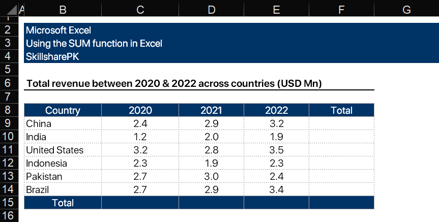
Suppose you have the data on total revenue between 2020 and 2022 given between cells B8 and F15, as shown in the table below, and you want to compute the total revenue generated for each country and in each year. You can add the numbers using the SUM function.

Recall that to use the SUM function, you will need to specify the range of cells that you want to add up and separate them with a comma.
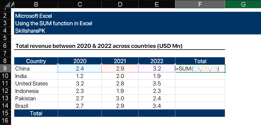
Here is how you can calculate the total revenue generated by China in the 3 years using the SUM function. Data for China is given in the cells D9, E9, and F9.
=SUM(C9,D9,E9)
This function will add up the values in cells C9, D9, and E9.

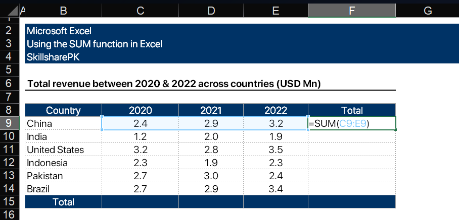
Alternatively, you can specify the range to the abovementioned cells. Enter the following formula in cell F9:
=SUM(C9:E9)
This function will add up all of the values in the range C9:E9.

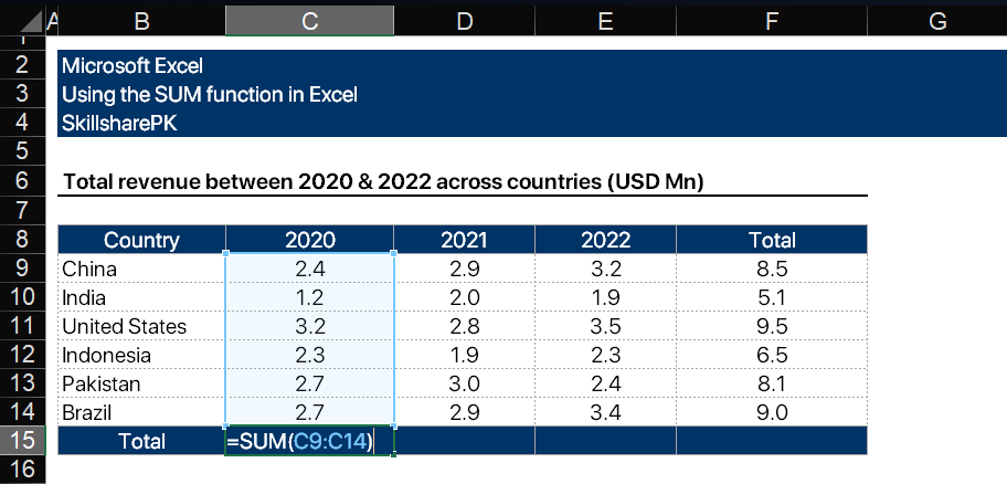
Now suppose that you want to compute the total revenue for each year. For our example, we are computing the total revenue in 2020, and data for the year 2020 is given in column C, between cells C9 and C15. We can accomplish this by using the SUM function and applying it in cell E15.
=SUM(C9:C15)

Moreover, you can also use the SUM function to add up values in multiple rows or columns by specifying a range that includes all of these cells. For example, if you want to add the total revenue in each year and each country, you can SUM all the cells in the entire range, C9 till F14.
=SUM(C9:E14)
This will add the values in the cells C9, C10, C11, C12, C13, C14, D9, D10, D11, D12, D13, D14, E9, E10, E11, E12, E13, and E14. See the picture below:

Alternatively, you can simply add the values in column F or row 15, using the SUM function. In that case, you can use the following formulas:
=SUM(C15:E15);
=SUM(F9:F14)
” content_phone=”
An example of using the sum function in Excel
Suppose you have the data on total revenue between 2020 and 2022 given between cells B8 and F15, as shown in the table below, and you want to compute the total revenue generated for each country and in each year. You can add the numbers using the SUM function.
Recall that to use the SUM function, you will need to specify the range of cells that you want to add up and separate them with a comma.
Here is how you can calculate the total revenue generated by China in the 3 years using the SUM function. Data for China is given in the cells D9, E9, and F9.
=SUM(C9,D9,E9)
This function will add up the values in cells C9, D9, and E9.
Alternatively, you can specify the range to the abovementioned cells. Enter the following formula in cell F9:
=SUM(C9:E9)
This function will add up all of the values in the range C9:E9.
Now suppose that you want to compute the total revenue for each year. For our example, we are computing the total revenue in 2020, and data for the year 2020 is given in column C, between cells C9 and C15. We can accomplish this by using the SUM function and applying it in cell E15.
=SUM(C9:C15)
Moreover, you can also use the SUM function to add up values in multiple rows or columns by specifying a range that includes all of these cells. For example, if you want to add the total revenue in each year and each country, you can SUM all the cells in the entire range, C9 till F14.
=SUM(C9:E14)
This will add the values in the cells C9, C10, C11, C12, C13, C14, D9, D10, D11, D12, D13, D14, E9, E10, E11, E12, E13, and E14. See the picture below:
Alternatively, you can simply add the values in column F or row 15, using the SUM function. In that case, you can use the following formulas:
=SUM(C15:E15);
=SUM(F9:F14)
” content_last_edited=”on|phone” _builder_version=”4.6.6″ _module_preset=”default” text_font=”Poppins|300|||||||” text_font_size=”16px” text_line_height=”1.8em” header_2_font=”Montserrat|800||on|||||” header_2_text_color=”#000000″ header_3_font=”Poppins|800|||||||” header_3_font_size=”16px” header_3_font_tablet=”” header_3_font_phone=”” header_3_font_last_edited=”on|phone”]
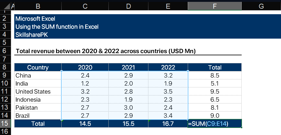
An example of using the sum function in Excel
Suppose you have the data on total revenue between 2020 and 2022 given between cells B8 and F15, as shown in the table below, and you want to compute the total revenue generated for each country and in each year. You can add the numbers using the SUM function.
Recall that to use the SUM function, you will need to specify the range of cells that you want to add up and separate them with a comma.
Here is how you can calculate the total revenue generated by China in the 3 years using the SUM function. Data for China is given in the cells D9, E9, and F9.
=SUM(C9,D9,E9)
This function will add up the values in cells C9, D9, and E9.
Alternatively, you can specify the range to the abovementioned cells. Enter the following formula in cell F9:
=SUM(C9:E9)
This function will add up all of the values in the range C9:E9.
Now suppose that you want to compute the total revenue for each year. For our example, we are computing the total revenue in 2020, and data for the year 2020 is given in column C, between cells C9 and C15. We can accomplish this by using the SUM function and applying it in cell E15.
=SUM(C9:C15)
Moreover, you can also use the SUM function to add up values in multiple rows or columns by specifying a range that includes all of these cells. For example, if you want to add the total revenue in each year and each country, you can SUM all the cells in the entire range, C9 till F14.
=SUM(C9:E14)
This will add the values in the cells C9, C10, C11, C12, C13, C14, D9, D10, D11, D12, D13, D14, E9, E10, E11, E12, E13, and E14. See the picture below:
Alternatively, you can simply add the values in column F or row 15, using the SUM function. In that case, you can use the following formulas:
=SUM(C15:E15);
=SUM(F9:F14)
[/et_pb_text][et_pb_text content_tablet=”
Follow us on our social media platforms:
” content_phone=”
Follow us on our social media platforms:
” content_last_edited=”on|tablet” _builder_version=”4.6.6″ _module_preset=”default” text_font=”Poppins|300|||||||” text_font_size=”16px” text_line_height=”1.8em” header_2_font=”Montserrat|800||on|||||” header_2_text_color=”#000000″ header_3_font=”Poppins|800|||||||” header_3_font_size=”16px” header_3_font_tablet=”” header_3_font_phone=”” header_3_font_last_edited=”on|phone”]
Follow us on our social media platforms:
[/et_pb_text][/et_pb_column][/et_pb_row][/et_pb_section]
Pingback: Using the SUMIF Function in Excel - Guide & Example