

[et_pb_section fb_built=”1″ _builder_version=”4.6.6″ _module_preset=”default”][et_pb_row _builder_version=”4.6.6″ _module_preset=”default”][et_pb_column type=”4_4″ _builder_version=”4.6.6″ _module_preset=”default”][et_pb_text content_tablet=”
How to use the VLOOKUP function?
” content_phone=”
How to use the VLOOKUP function?
” content_last_edited=”on|desktop” _builder_version=”4.6.6″ _module_preset=”default” header_font=”Montserrat|800||on|||||” header_text_color=”#000000″ hover_enabled=”0″ sticky_enabled=”0″]
How to use the VLOOKUP function?
[/et_pb_text][et_pb_text content_tablet=”
VLOOKUP is a built-in Excel function that allows you to search for a specific value in a range of cells and return a corresponding value from a different column in the same row. It is a useful tool for looking up and retrieving data from large tables of data or databases.
” content_phone=”
VLOOKUP is a built-in Excel function that allows you to search for a specific value in a range of cells and return a corresponding value from a different column in the same row. It is a useful tool for looking up and retrieving data from large tables of data or databases.
” content_last_edited=”on|phone” _builder_version=”4.6.6″ _module_preset=”default” text_font=”Poppins|300|||||||” text_font_size=”16px” text_line_height=”1.8em” header_2_font=”Montserrat|800||on|||||”]
VLOOKUP is a built-in Excel function that allows you to search for a specific value in a range of cells and return a corresponding value from a different column in the same row. It is a useful tool for looking up and retrieving data from large tables of data or databases.
[/et_pb_text][et_pb_image src=”http://skillsharepk.com/wp-content/uploads/2022/12/Vlookup-1.jpg” alt=”Using the Vlookup function” title_text=”Vlookup” _builder_version=”4.6.6″ _module_preset=”default”][/et_pb_image][/et_pb_column][/et_pb_row][et_pb_row _builder_version=”4.6.6″ _module_preset=”default”][et_pb_column type=”4_4″ _builder_version=”4.6.6″ _module_preset=”default”][et_pb_text content_tablet=”
VLOOKUP is arguably Excel’s most well-known function, It has both pros and cons to it. On the plus side, it is simple to use and helps in performing an essential tasks quite. It’s intriguing for beginner Excel users to see VLOOKUP scan a table, identify a match, and provide the proper result.
That said, VLOOKUP does have its shortcomings. Firstly, unlike some of its alternatives (including the INDEX and MATCH, or XLOOKUP), VLOOKUP works only when the lookup values are in the first column. This makes using it with multiple criteria difficult. Furthermore, the default matching behavior of VLOOKUP makes it easy to obtain inaccurate results (we’ll discuss this ahead). Nevertheless, we’ll cover it all in detail so that you are well aware of the syntax and can apply the VLOOKUP function successfully. Continue reading for a comprehensive overview.
” content_phone=”
VLOOKUP is arguably Excel’s most well-known function, It has both pros and cons to it. On the plus side, it is simple to use and helps in performing an essential tasks quite. It’s intriguing for beginner Excel users to see VLOOKUP scan a table, identify a match, and provide the proper result.
That said, VLOOKUP does have its shortcomings. Firstly, unlike some of its alternatives (including the INDEX and MATCH, or XLOOKUP), VLOOKUP works only when the lookup values are in the first column. This makes using it with multiple criteria difficult. Furthermore, the default matching behavior of VLOOKUP makes it easy to obtain inaccurate results (we’ll discuss this ahead). Nevertheless, we’ll cover it all in detail so that you are well aware of the syntax and can apply the VLOOKUP function successfully. Continue reading for a comprehensive overview.
” content_last_edited=”on|phone” _builder_version=”4.6.6″ _module_preset=”default” text_font=”Poppins|300|||||||” text_font_size=”16px” text_line_height=”1.8em” header_3_font=”Montserrat|800||on|||||”]
VLOOKUP is arguably Excel’s most well-known function, It has both pros and cons to it. On the plus side, it is simple to use and helps in performing an essential tasks quite. It’s intriguing for beginner Excel users to see VLOOKUP scan a table, identify a match, and provide the proper result.
That said, VLOOKUP does have its shortcomings. Firstly, unlike some of its alternatives (including the INDEX and MATCH, or XLOOKUP), VLOOKUP works only when the lookup values are in the first column. This makes using it with multiple criteria difficult. Furthermore, the default matching behavior of VLOOKUP makes it easy to obtain inaccurate results (we’ll discuss this ahead). Nevertheless, we’ll cover it all in detail so that you are well aware of the syntax and can apply the VLOOKUP function successfully. Continue reading for a comprehensive overview.
[/et_pb_text][et_pb_text content_tablet=”
How to use the VLOOKUP function on Excel?
Firstly, remember that VLOOKUP is used when looking at information in vertical columns. To be more specific, the VLOOKUP function is used when you want to search for a specific value in a range of cells and return a corresponding value from a different column in the same row.
To use the data that is in horizontal rows, use the HLOOKUP, INDEX & MATCH, or XLOOKUP functions.
However, for our article, let’s focus on VLOOKUP.
There are four inputs that you need to give to write the VLOOKUP formula. Here is the syntax for the VLOOKUP function:
=VLOOKUP(lookup_value, table_array, col_index_number, %91range_lookup%93)
- lookup_value: what you want to look up (the value against which you want a corresponding value)
- table_arry: this is the range of cells that contain the data that you want to search through
- column_index_number: this is the column number in the table from which the VLOOKUP function gets the returning value
- range_lookup: this controls the matching behavior. VLOOKUP will find an approximate match if the range lookup is TRUE. On the other hand, VLOOKUP will find an exact match if the range lookup is set to FALSE. Note that range lookup is an optional parameter with the default value as TRUE, implying that VLOOKUP will execute an approximate match by default. Therefore, you must enter FALSE (or 0) if you want an exact match
” content_phone=”
How to use the VLOOKUP function on Excel?
Firstly, remember that VLOOKUP is used when looking at information in vertical columns. To be more specific, the VLOOKUP function is used when you want to search for a specific value in a range of cells and return a corresponding value from a different column in the same row.
To use the data that is in horizontal rows, use the HLOOKUP, INDEX & MATCH, or XLOOKUP functions.
However, for our article, let’s focus on VLOOKUP.
There are four inputs that you need to give to write the VLOOKUP formula. Here is the syntax for the VLOOKUP function:
=VLOOKUP(lookup_value, table_array, col_index_number, %91range_lookup%93)
- lookup_value: what you want to look up (the value against which you want a corresponding value)
- table_arry: this is the range of cells that contain the data that you want to search through
- column_index_number: this is the column number in the table from which the VLOOKUP function gets the returning value
- range_lookup: this controls the matching behavior. VLOOKUP will find an approximate match if the range lookup is TRUE. On the other hand, VLOOKUP will find an exact match if the range lookup is set to FALSE. Note that range lookup is an optional parameter with the default value as TRUE, implying that VLOOKUP will execute an approximate match by default. Therefore, you must enter FALSE (or 0) if you want an exact match
” content_last_edited=”on|phone” _builder_version=”4.6.6″ _module_preset=”default” text_font=”Poppins|300|||||||” text_font_size=”16px” text_line_height=”1.8em” header_font=”Poppins|800|||||||” header_2_font=”Montserrat|800||on|||||” header_2_text_color=”#000000″ header_3_font=”Poppins|800|||||||” header_3_font_size=”16px” header_2_font_tablet=”” header_2_font_phone=”” header_2_font_last_edited=”on|phone” header_3_font_tablet=”” header_3_font_phone=”” header_3_font_last_edited=”on|tablet”]
How to use the VLOOKUP function on Excel?
Firstly, remember that VLOOKUP is used when looking at information in vertical columns. To be more specific, the VLOOKUP function is used when you want to search for a specific value in a range of cells and return a corresponding value from a different column in the same row.
To use the data that is in horizontal rows, use the HLOOKUP, INDEX & MATCH, or XLOOKUP functions.
However, for our article, let’s focus on VLOOKUP.
There are four inputs that you need to give to write the VLOOKUP formula. Here is the syntax for the VLOOKUP function:
=VLOOKUP(lookup_value, table_array, col_index_number, [range_lookup])
- lookup_value: what you want to look up (the value against which you want a corresponding value)
- table_arry: this is the range of cells that contain the data that you want to search through
- column_index_number: this is the column number in the table from which the VLOOKUP function gets the returning value
- range_lookup: this controls the matching behavior. VLOOKUP will find an approximate match if the range lookup is TRUE. On the other hand, VLOOKUP will find an exact match if the range lookup is set to FALSE. Note that range lookup is an optional parameter with the default value as TRUE, implying that VLOOKUP will execute an approximate match by default. Therefore, you must enter FALSE (or 0) if you want an exact match
[/et_pb_text][et_pb_text content_tablet=”
Here is how you apply the VLOOKUP function on Excel
- In the cell where you want to display the result of the VLOOKUP function, type ‘=VLOOKUP’ and start the function by opening the parentheses.
- After selecting the lookup value, type a comma (,) and proceed to the second argument. Now choose the range of cells that contain the data that you want to search through
- Enter a comma (,) again, and then enter the number of the column in the range of cells that contains the value you want to return.
- Finally, type another comma and then specify whether you want an exact or an approximate match. Enter FALSE or 0 to specify an exact match. Enter TRUE or 1 to signify an approximate match.
- To finish the formula, press Enter. The VLOOKUP function will look up the lookup value in the provided range of cells and return the value from the specified column in the same row.
” content_phone=”
Here is how you apply the VLOOKUP function on Excel
- In the cell where you want to display the result of the VLOOKUP function, type ‘=VLOOKUP’ and start the function by opening the parentheses.
- After selecting the lookup value, type a comma (,) and proceed to the second argument. Now choose the range of cells that contain the data that you want to search through
- Enter a comma (,) again, and then enter the number of the column in the range of cells that contains the value you want to return.
- Finally, type another comma and then specify whether you want an exact or an approximate match. Enter FALSE or 0 to specify an exact match. Enter TRUE or 1 to signify an approximate match.
- To finish the formula, press Enter. The VLOOKUP function will look up the lookup value in the provided range of cells and return the value from the specified column in the same row.
” content_last_edited=”on|desktop” _builder_version=”4.6.6″ _module_preset=”default” text_font=”Poppins|300|||||||” text_font_size=”16px” text_line_height=”1.8em” header_2_font=”Montserrat|800||on|||||” header_2_text_color=”#000000″ header_3_font=”Poppins|800|||||||” header_3_font_size=”16px” header_3_font_tablet=”” header_3_font_phone=”” header_3_font_last_edited=”on|phone”]
Here is how you apply the VLOOKUP function on Excel
- In the cell where you want to display the result of the VLOOKUP function, type ‘=VLOOKUP’ and start the function by opening the parentheses.
- After selecting the lookup value, type a comma (,) and proceed to the second argument. Now choose the range of cells that contain the data that you want to search through
- Enter a comma (,) again, and then enter the number of the column in the range of cells that contains the value you want to return.
- Finally, type another comma and then specify whether you want an exact or an approximate match. Enter FALSE or 0 to specify an exact match. Enter TRUE or 1 to signify an approximate match.
- To finish the formula, press Enter. The VLOOKUP function will look up the lookup value in the provided range of cells and return the value from the specified column in the same row.
[/et_pb_text][et_pb_text content_tablet=”
Example of using VLOOKUP function on Excel
Suppose you have the following data table for the top 10 countries in the world by Population:
%91caption id=%22attachment_1555%22 align=%22aligncenter%22 width=%22857%22%93
Now, suppose you want to extract the Population size of Pakistan in a certain cell.
So this is the formula that you will enter:
=VLOOKUP(A6, A2:F11,2,0)
In addition, be careful that you anchor the cells and the range so the VLOOKUP function can be easily replicated.
The function will then look like this:
=VLOOKUP(A6, $A$2:$F$11,2,0)
This formula searches for the value %22Pakistan%22 in the first column of the table (column A), and returns the corresponding value in the second column (column B), which is %22220,892,340%22.
Let’s try another example of the VLOOKUP function. Suppose you want to extract the Fertility rate of China. So this time, you will enter the following formula:
=VLOOKUP(A2, A2:F11,6,0)
This formula searches for the value %22China%22 in the first column of the table (column A) and returns the corresponding value in the sixth column (column F), which is %221.7%22.
” content_phone=”
Example of using VLOOKUP function on Excel
Suppose you have the following data table for the top 10 countries in the world by Population:
%91caption id=%22attachment_1555%22 align=%22aligncenter%22 width=%22857%22%93 Source: https://www.worldometers.info/world-population/population-by-country/%91/caption%93
Now, suppose you want to extract the Population size of Pakistan in a certain cell.
So this is the formula that you will enter:
=VLOOKUP(A6, A2:F11,2,0)
In addition, be careful that you anchor the cells and the range so the VLOOKUP function can be easily replicated.
The function will then look like this:
=VLOOKUP(A6, $A$2:$F$11,2,0)
This formula searches for the value %22Pakistan%22 in the first column of the table (column A), and returns the corresponding value in the second column (column B), which is %22220,892,340%22.
Let’s try another example of the VLOOKUP function. Suppose you want to extract the Fertility rate of China. So this time, you will enter the following formula:
=VLOOKUP(A2, A2:F11,6,0)
This formula searches for the value %22China%22 in the first column of the table (column A) and returns the corresponding value in the sixth column (column F), which is %221.7%22.
” content_last_edited=”on|phone” _builder_version=”4.6.6″ _module_preset=”default” text_font=”Poppins|300|||||||” text_font_size=”16px” text_line_height=”1.8em” header_2_font=”Montserrat|800||on|||||” header_2_text_color=”#000000″ header_3_font=”Poppins|800|||||||” header_3_font_size=”16px” header_3_font_tablet=”” header_3_font_phone=”” header_3_font_last_edited=”on|phone”]
Example of using VLOOKUP function on Excel
Suppose you have the following data table for the top 10 countries in the world by Population:
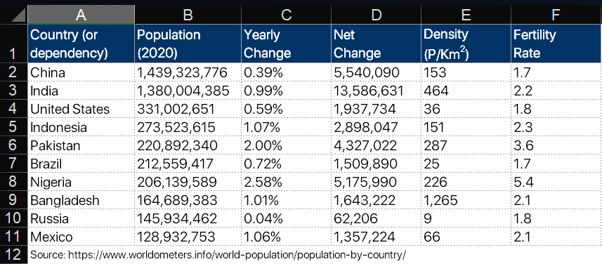
Now, suppose you want to extract the Population size of Pakistan in a certain cell.
So this is the formula that you will enter:
=VLOOKUP(A6, A2:F11,2,0)
In addition, be careful that you anchor the cells and the range so the VLOOKUP function can be easily replicated.
The function will then look like this:
=VLOOKUP(A6, $A$2:$F$11,2,0)
This formula searches for the value “Pakistan” in the first column of the table (column A), and returns the corresponding value in the second column (column B), which is “220,892,340“.
Let’s try another example of the VLOOKUP function. Suppose you want to extract the Fertility rate of China. So this time, you will enter the following formula:
=VLOOKUP(A2, A2:F11,6,0)
This formula searches for the value “China” in the first column of the table (column A) and returns the corresponding value in the sixth column (column F), which is “1.7“.
[/et_pb_text][et_pb_text content_tablet=”
Follow us on our social media platforms:
” content_phone=”
Follow us on our social media platforms:
” content_last_edited=”on|tablet” _builder_version=”4.6.6″ _module_preset=”default” text_font=”Poppins|300|||||||” text_font_size=”16px” text_line_height=”1.8em” header_2_font=”Montserrat|800||on|||||” header_2_text_color=”#000000″ header_3_font=”Poppins|800|||||||” header_3_font_size=”16px” header_3_font_tablet=”” header_3_font_phone=”” header_3_font_last_edited=”on|phone”]
Follow us on our social media platforms:
[/et_pb_text][/et_pb_column][/et_pb_row][/et_pb_section]