

[et_pb_section fb_built=”1″ _builder_version=”4.6.6″ _module_preset=”default”][et_pb_row _builder_version=”4.6.6″ _module_preset=”default”][et_pb_column type=”4_4″ _builder_version=”4.6.6″ _module_preset=”default”][et_pb_text content_last_edited=”off|desktop” _builder_version=”4.6.6″ _module_preset=”default” header_font=”Montserrat|800||on|||||” header_text_color=”#000000″]
Using the SUMIF Function in EXCEL – Guide & Example
[/et_pb_text][et_pb_text content_tablet=”
The SUMIF function in Excel is used to sum up a range of cells that fulfil certain criteria. It is a useful tool for summarizing and adding data based on specified conditions.
Earlier, we wrote about how to use the IF and SUM functions in Excel. The SUMIF function practically combines the two Excel functions so that you can add up values based on certain criteria or logic.
For instance, if you have a spreadsheet with a dataset that contains sales data across different regions and different periods, you can use the SUMIF function to find the total sales for a specific region. We will come back to this example of using the SUMIF function later.
” content_phone=”
The SUMIF function in Excel is used to sum up a range of cells that fulfil certain criteria. It is a useful tool for summarizing and adding data based on specified conditions.
Earlier, we wrote about how to use the IF and SUM functions in Excel. The SUMIF function practically combines the two Excel functions so that you can add up values based on certain criteria or logic.
For instance, if you have a spreadsheet with a dataset that contains sales data across different regions and different periods, you can use the SUMIF function to find the total sales for a specific region. We will come back to this example of using the SUMIF function later.
” content_last_edited=”on|desktop” _builder_version=”4.6.6″ _module_preset=”default” text_font=”Poppins|300|||||||” text_font_size=”16px” text_line_height=”1.8em”]
The SUMIF function in Excel is used to sum up a range of cells that fulfil certain criteria. It is a useful tool for summarizing and adding data based on specified conditions.
Earlier, we wrote about how to use the IF and SUM functions in Excel. The SUMIF function practically combines the two Excel functions so that you can add up values based on certain criteria or logic.
For instance, if you have a spreadsheet with a dataset that contains sales data across different regions and different periods, you can use the SUMIF function to find the total sales for a specific region. We will come back to this example of using the SUMIF function later.
[/et_pb_text][et_pb_image src=”http://skillsharepk.com/wp-content/uploads/2023/01/SUMIF.jpg” alt=”Using the SUMIF Function” title_text=”Using the SUMIF Function” _builder_version=”4.6.6″ _module_preset=”default” border_width_all=”1px” border_color_all=”#d8d8d8″][/et_pb_image][/et_pb_column][/et_pb_row][et_pb_row _builder_version=”4.6.6″ _module_preset=”default”][et_pb_column type=”4_4″ _builder_version=”4.6.6″ _module_preset=”default”][et_pb_text content_tablet=”
Using the SUMIF Function in Excel
Here is the syntax to use the SUMIF function:
%91su_note note_color=%22#b0def9%22%93=SUMIF(range, criteria, %91sum_range%93)%91/su_note%93
- range: the cells that you want to apply the criteria to.
- criteria: the logic or the criteria must meet to be included in the sum
- sum_range: an optional argument that specifies the range of cells to sum given the criteria specified earlier. If this argument is left blank, Excel will sum the cells in the range specified in the range argument.
For example, suppose you have a list of values in the cell range A1:A10, and you want to add up only the values that are greater than 10. You can do that using the SUMIF formula below:
%91su_note note_color=%22#b0def9%22%93=SUMIF(A1:A10, %22>5%22)%91/su_note%93
This would sum up the values in A1:A10 that are greater than 10.
Moreover, the SUMIF function can also be used to sum up values based on a specific text. For example, suppose you have a list of names in column A and a list of numeric values in column B, and you want to sum the values in column B for all the cells in column A that contain the name %22Muhammad%22. You could use the following formula:
%91su_note note_color=%22#b0def9%22%93=SUMIF(A1:A10, %22Muhammad%22, B1:B10)%91/su_note%93
This would sum the values in B1:B10 for all the cells in A1:A10 that contain the name %22Muhammad%22.
Remember, while entering the criteria, make sure that you put it in an enclosed bracket (“ ”)
” content_phone=”
Using the SUMIF Function in Excel
Here is the syntax to use the SUMIF function:
%91su_note note_color=%22#b0def9%22%93=SUMIF(range, criteria, %91sum_range%93)%91/su_note%93
- range: the cells that you want to apply the criteria to.
- criteria: the logic or the criteria must meet to be included in the sum
- sum_range: an optional argument that specifies the range of cells to sum given the criteria specified earlier. If this argument is left blank, Excel will sum the cells in the range specified in the range argument.
For example, suppose you have a list of values in the cell range A1:A10, and you want to add up only the values that are greater than 10. You can do that using the SUMIF formula below:
%91su_note note_color=%22#b0def9%22%93=SUMIF(A1:A10, %22>5%22)%91/su_note%93
This would sum up the values in A1:A10 that are greater than 10.
Moreover, the SUMIF function can also be used to sum up values based on a specific text. For example, suppose you have a list of names in column A and a list of numeric values in column B, and you want to sum the values in column B for all the cells in column A that contain the name %22Muhammad%22. You could use the following formula:
%91su_note note_color=%22#b0def9%22%93=SUMIF(A1:A10, %22Muhammad%22, B1:B10)%91/su_note%93
This would sum the values in B1:B10 for all the cells in A1:A10 that contain the name %22Muhammad%22.
Remember, while entering the criteria, make sure that you put it in an enclosed bracket (“ ”)
” content_last_edited=”on|desktop” _builder_version=”4.6.6″ _module_preset=”default” text_font=”Poppins|300|||||||” text_font_size=”16px” text_line_height=”1.8em” header_font=”Poppins|800|||||||” header_2_font=”Montserrat|800||on|||||” header_2_text_color=”#000000″ header_3_font=”Poppins|800|||||||” header_3_font_size=”16px” header_2_font_tablet=”” header_2_font_phone=”” header_2_font_last_edited=”on|phone” header_3_font_tablet=”” header_3_font_phone=”” header_3_font_last_edited=”on|tablet”]
Using the SUMIF Function in Excel
Here is the syntax to use the SUMIF function:
[su_note note_color=”#b0def9″]=SUMIF(range, criteria, [sum_range])[/su_note]
- range: the cells that you want to apply the criteria to.
- criteria: the logic or the criteria must meet to be included in the sum
- sum_range: an optional argument that specifies the range of cells to sum given the criteria specified earlier. If this argument is left blank, Excel will sum the cells in the range specified in the range argument.
For example, suppose you have a list of values in the cell range A1:A10, and you want to add up only the values that are greater than 10. You can do that using the SUMIF formula below:
[su_note note_color=”#b0def9″]=SUMIF(A1:A10, “>5”)[/su_note]
This would sum up the values in A1:A10 that are greater than 10.
Moreover, the SUMIF function can also be used to sum up values based on a specific text. For example, suppose you have a list of names in column A and a list of numeric values in column B, and you want to sum the values in column B for all the cells in column A that contain the name “Muhammad”. You could use the following formula:
[su_note note_color=”#b0def9″]=SUMIF(A1:A10, “Muhammad”, B1:B10)[/su_note]
This would sum the values in B1:B10 for all the cells in A1:A10 that contain the name “Muhammad“.
Remember, while entering the criteria, make sure that you put it in an enclosed bracket (“ ”)
[/et_pb_text][et_pb_text content_tablet=”
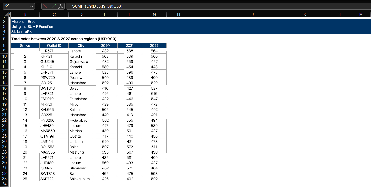
An example of using the SUMIF function
Suppose you have data on total sales made by a company between 2020 and 2022
%91caption id=%22attachment_1806%22 align=%22aligncenter%22 width=%221457%22%93
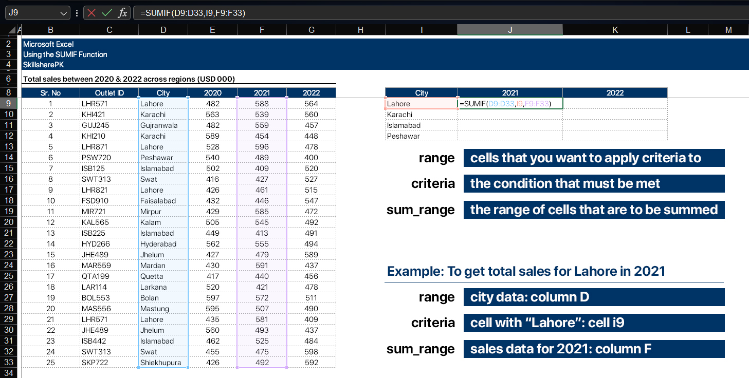
Now suppose you want to find the total sales made in Lahore in 2021. You can easily calculate this using the SUMIF function shown below:
%91su_note note_color=%22#b0def9%22%93=SUMIF(D9:D33, I9, F9:F33)%91/su_note%93
To elaborate, the ‘range’ is defined in column D (containing data on cities), the ‘criteria’ is given in cell I9 (Lahore) and the values to be added i.e. the ‘sum range’ is given in column F (data on sales)

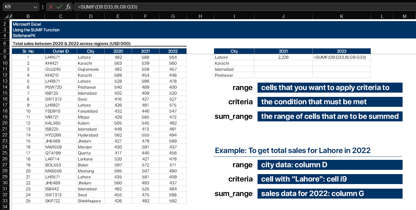
Similarly, if you want to calculate the total sales in Lahore in the year 2022: You can once again accomplish that using the SUMIF function as shown below:
%91su_note note_color=%22#b0def9%22%93=SUMIF(D9:D33, I9, G9:G33)%91/su_note%93
In this case, ‘range’ is defined in column D (containing data on cities), the ‘criteria’ is given in cell I9 (Lahore) and the values to be added i.e. the ‘sum range’ is given in column G (data on sales)

But what if you want to apply multiple conditions? In that case, you can achieve that using the SUMIFS function.
” content_phone=”
An example of using the SUMIF function
Suppose you have data on total sales made by a company between 2020 and 2022
%91caption id=%22attachment_1806%22 align=%22aligncenter%22 width=%221457%22%93 Total sales between 2020 and 2022%91/caption%93
Now suppose you want to find the total sales made in Lahore in 2021. You can easily calculate this using the SUMIF function shown below:
%91su_note note_color=%22#b0def9%22%93=SUMIF(D9:D33, I9, F9:F33)%91/su_note%93
To elaborate, the ‘range’ is defined in column D (containing data on cities), the ‘criteria’ is given in cell I9 (Lahore) and the values to be added i.e. the ‘sum range’ is given in column F (data on sales)
Similarly, if you want to calculate the total sales in Lahore in the year 2022: You can once again accomplish that using the SUMIF function as shown below:
%91su_note note_color=%22#b0def9%22%93=SUMIF(D9:D33, I9, G9:G33)%91/su_note%93
In this case, ‘range’ is defined in column D (containing data on cities), the ‘criteria’ is given in cell I9 (Lahore) and the values to be added i.e. the ‘sum range’ is given in column G (data on sales)
But what if you want to apply multiple conditions? In that case, you can achieve that using the SUMIFS function.
” content_last_edited=”on|phone” _builder_version=”4.6.6″ _module_preset=”default” text_font=”Poppins|300|||||||” text_font_size=”16px” text_line_height=”1.8em” header_2_font=”Montserrat|800||on|||||” header_2_text_color=”#000000″ header_3_font=”Poppins|800|||||||” header_3_font_size=”16px” header_3_font_tablet=”” header_3_font_phone=”” header_3_font_last_edited=”on|phone”]
An example of using the SUMIF function
Suppose you have data on total sales made by a company between 2020 and 2022
Now suppose you want to find the total sales made in Lahore in 2021. You can easily calculate this using the SUMIF function shown below:
[su_note note_color=”#b0def9″]=SUMIF(D9:D33, I9, F9:F33)[/su_note]
To elaborate, the ‘range’ is defined in column D (containing data on cities), the ‘criteria’ is given in cell I9 (Lahore) and the values to be added i.e. the ‘sum range’ is given in column F (data on sales)
Similarly, if you want to calculate the total sales in Lahore in the year 2022: You can once again accomplish that using the SUMIF function as shown below:
[su_note note_color=”#b0def9″]=SUMIF(D9:D33, I9, G9:G33)[/su_note]
In this case, ‘range’ is defined in column D (containing data on cities), the ‘criteria’ is given in cell I9 (Lahore) and the values to be added i.e. the ‘sum range’ is given in column G (data on sales)
But what if you want to apply multiple conditions? In that case, you can achieve that using the SUMIFS function.
[/et_pb_text][et_pb_text content_tablet=”
Using the SUMIFS Function
The SUMIFS function is practically the same as the SUMIF function, except that you can define multiple criteria and conditions within the same function.
The syntax for the SUMIFS function is as below:
%91su_note note_color=%22#b0def9%22%93SUMIFS(sum_range, criteria_range1, criteria1, %91criteria_range2, criteria2%93…)%91/su_note%93
- sum_range is the range of cells that you want to sum
- criteria_range1, criteria_range2, etc. are the ranges of cells that you want to use as criteria to determine which cells in the sum_range to add
- criteria1, criteria2, etc. are the conditions that you want to use to filter the criteria_range1, criteria_range2
Note that the second criterion is an optional input, and is therefore given in a square bracket (%91 %93). Finally, you can add as many conditions as you want using the SUMIFS function.
” content_phone=”
Using the SUMIFS Function
The SUMIFS function is practically the same as the SUMIF function, except that you can define multiple criteria and conditions within the same function.
The syntax for the SUMIFS function is as below:
%91su_note note_color=%22#b0def9%22%93SUMIFS(sum_range, criteria_range1, criteria1, %91criteria_range2, criteria2%93…)%91/su_note%93
- sum_range is the range of cells that you want to sum
- criteria_range1, criteria_range2, etc. are the ranges of cells that you want to use as criteria to determine which cells in the sum_range to add
- criteria1, criteria2, etc. are the conditions that you want to use to filter the criteria_range1, criteria_range2
Note that the second criterion is an optional input, and is therefore given in a square bracket (%91 %93). Finally, you can add as many conditions as you want using the SUMIFS function.
” content_last_edited=”on|phone” _builder_version=”4.6.6″ _module_preset=”default” text_font=”Poppins|300|||||||” text_font_size=”16px” text_line_height=”1.8em” header_2_font=”Montserrat|800||on|||||” header_2_text_color=”#000000″ header_3_font=”Poppins|800|||||||” header_3_font_size=”16px” header_3_font_tablet=”” header_3_font_phone=”” header_3_font_last_edited=”on|phone”]
Using the SUMIFS Function
The SUMIFS function is practically the same as the SUMIF function, except that you can define multiple criteria and conditions within the same function.
The syntax for the SUMIFS function is as below:
[su_note note_color=”#b0def9″]SUMIFS(sum_range, criteria_range1, criteria1, [criteria_range2, criteria2]…)[/su_note]
- sum_range is the range of cells that you want to sum
- criteria_range1, criteria_range2, etc. are the ranges of cells that you want to use as criteria to determine which cells in the sum_range to add
- criteria1, criteria2, etc. are the conditions that you want to use to filter the criteria_range1, criteria_range2
Note that the second criterion is an optional input, and is therefore given in a square bracket ([ ]). Finally, you can add as many conditions as you want using the SUMIFS function.
[/et_pb_text][et_pb_text content_tablet=”
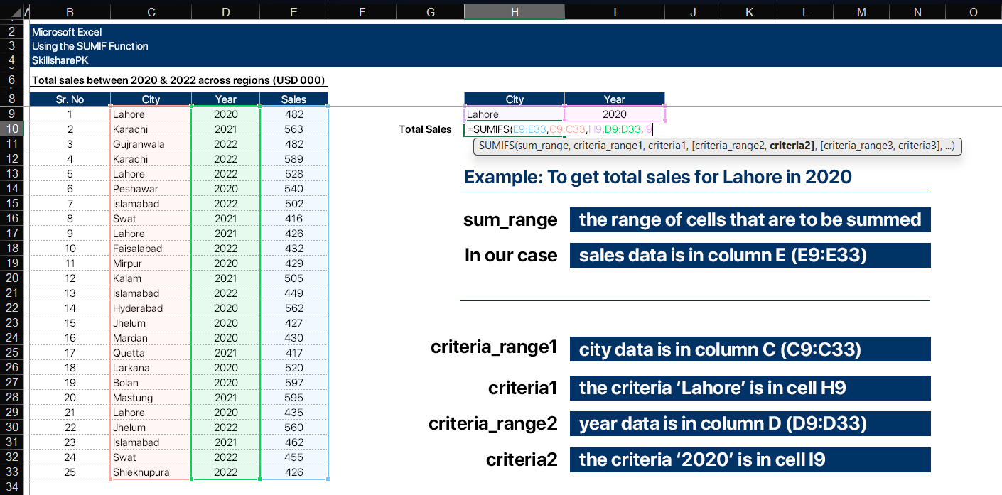
An Example of Using the SUMIFS Function
Suppose that instead of having data of sales across different columns, you have data within a single column. In such a case, you will have the use the SUMIFS function.
For example, to find our the total sales made in Lahore in the year 2020, you will enter the formula as in shown in the picture below:
%91caption id=%22attachment_1812%22 align=%22aligncenter%22 width=%221410%22%93 Enter multiple conditions within the same formula using the SUMIFS function%91/caption%93
” content_phone=”
An Example of Using the SUMIFS Function
Suppose that instead of having data of sales across different columns, you have data within a single column. In such a case, you will have the use the SUMIFS function.
For example, to find our the total sales made in Lahore in the year 2020, you will enter the formula as in shown in the picture below:
%91caption id=%22attachment_1812%22 align=%22aligncenter%22 width=%221410%22%93 Enter multiple conditions within the same formula using the SUMIFS function%91/caption%93
” content_last_edited=”on|desktop” _builder_version=”4.6.6″ _module_preset=”default” text_font=”Poppins|300|||||||” text_font_size=”16px” text_line_height=”1.8em” header_2_font=”Montserrat|800||on|||||” header_2_text_color=”#000000″ header_3_font=”Poppins|800|||||||” header_3_font_size=”16px” header_3_font_tablet=”” header_3_font_phone=”” header_3_font_last_edited=”on|phone”]
An Example of Using the SUMIFS Function
Suppose that instead of having data of sales across different columns, you have data within a single column. In such a case, you will have the use the SUMIFS function.
For example, to find our the total sales made in Lahore in the year 2020, you will enter the formula as in shown in the picture below:
[/et_pb_text][et_pb_text content_tablet=”
Follow us on our social media platforms:
” content_phone=”
Follow us on our social media platforms:
” content_last_edited=”on|desktop” _builder_version=”4.6.6″ _module_preset=”default” text_font=”Poppins|300|||||||” text_font_size=”16px” text_line_height=”1.8em” header_2_font=”Montserrat|800||on|||||” header_2_text_color=”#000000″ header_3_font=”Poppins|800|||||||” header_3_font_size=”16px” header_3_font_tablet=”” header_3_font_phone=”” header_3_font_last_edited=”on|phone” locked=”off”]
Follow us on our social media platforms:
[/et_pb_text][/et_pb_column][/et_pb_row][et_pb_row _builder_version=”4.6.6″ _module_preset=”default”][et_pb_column _builder_version=”4.6.6″ _module_preset=”default” type=”4_4″][et_pb_code _builder_version=”4.6.6″ _module_preset=”default” hover_enabled=”0″ sticky_enabled=”0″] style=”display:block” data-ad-client=”ca-pub-3376158381162076″ data-ad-slot=”5991215789″ data-ad-format=”auto” data-full-width-responsive=”true”>[/et_pb_code][et_pb_text _builder_version=”4.6.6″ _module_preset=”default” hover_enabled=”0″ sticky_enabled=”0″]
[/et_pb_text][/et_pb_column][/et_pb_row][/et_pb_section]